Modules
Six modules, one data model
Every module reads from and writes to the same project, so samples, PHREEQC results and derived data can be filtered, combined and plotted together. Community includes Akva and Phreeqc; Professional adds the other four.
Ak · Community
Akva
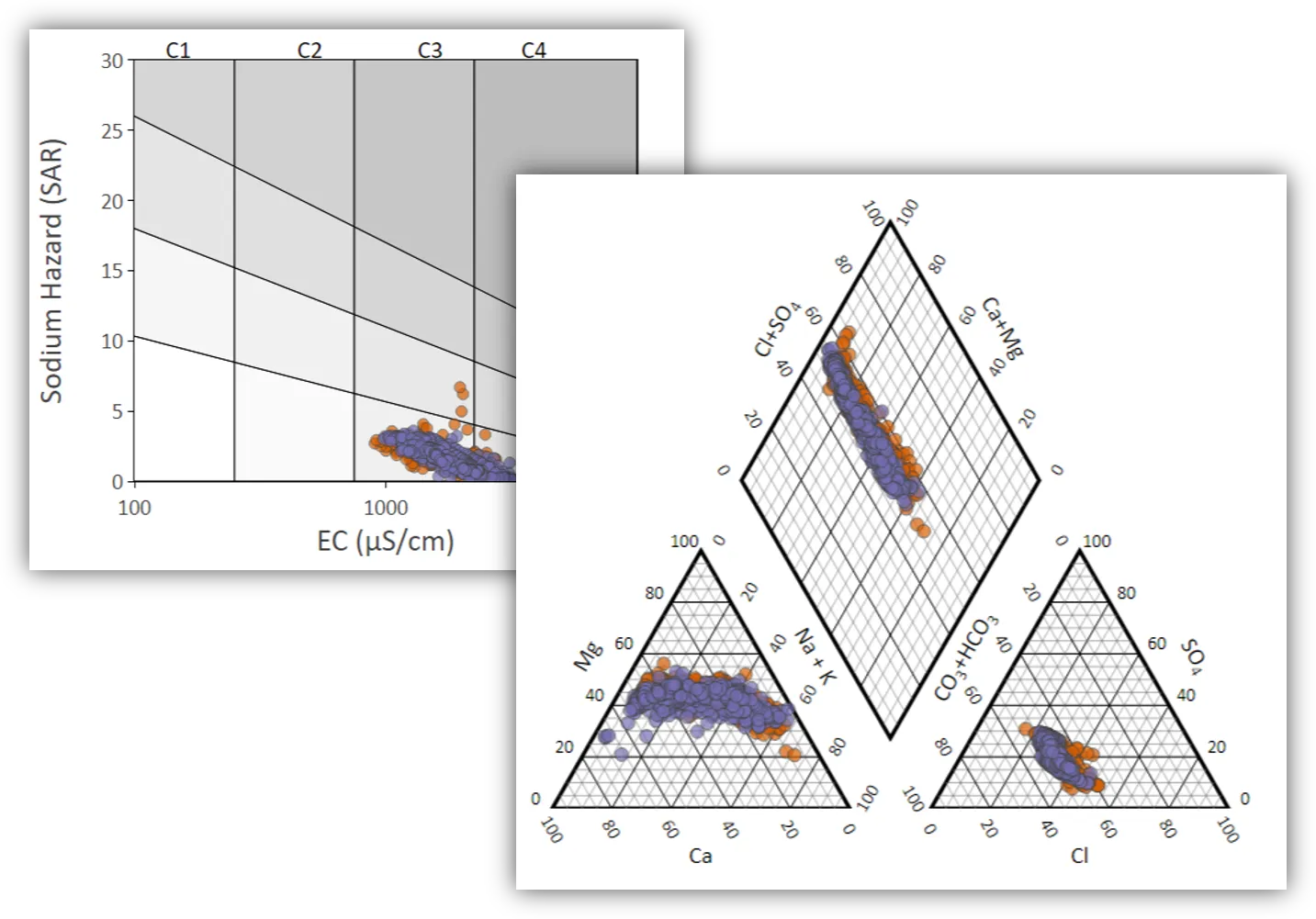
Water Chemistry — the Akva module — takes a table of water analyses and tells you whether each one is self-consistent, what kind of water it is, and whether it is fit for irrigation.
- Columns matched by name. Import analyses from CSV, tab-separated files or SQLite. Columns are found by name, not by position, so the order does not matter and extra columns are ignored. A blank or non-numeric cell is reported as missing rather than guessed at.
- The ion balance first. The charge balance error is computed from the eight major ions in meq/l, against the tolerance you set. A sample outside it stays in the table but can be left out of the aggregates and the diagrams.
- Water type, facies and irrigation indices. Each analysis is named by its dominant cation and anion and by its Piper facies, and scored with SAR, Na %, RSC, the Kelly ratio, magnesium hazard, permeability index, hardness and — with conductivity — the USSL class.
- Aggregate by point or category. Earliest, latest, minimum, maximum, mean or median, so you can ask what a spring is like rather than what one bottle was like. Each aggregate says how many samples it came from.
- Piper, Schoeller and USSL diagrams. The three diagrams hydrochemists expect, each available as a quick result that builds the plot and the analysis behind it in one step. Export to SVG, HTML or image formats.
- Samples next to model results. Plot field samples and PHREEQC results in the same figure, so calibration is a visual check instead of a spreadsheet exercise.
Pq · Community
Phreeqc
Run PHREEQC from a project that keeps inputs, databases, parameters and results together. PHREEQC is bundled, nothing else to install.
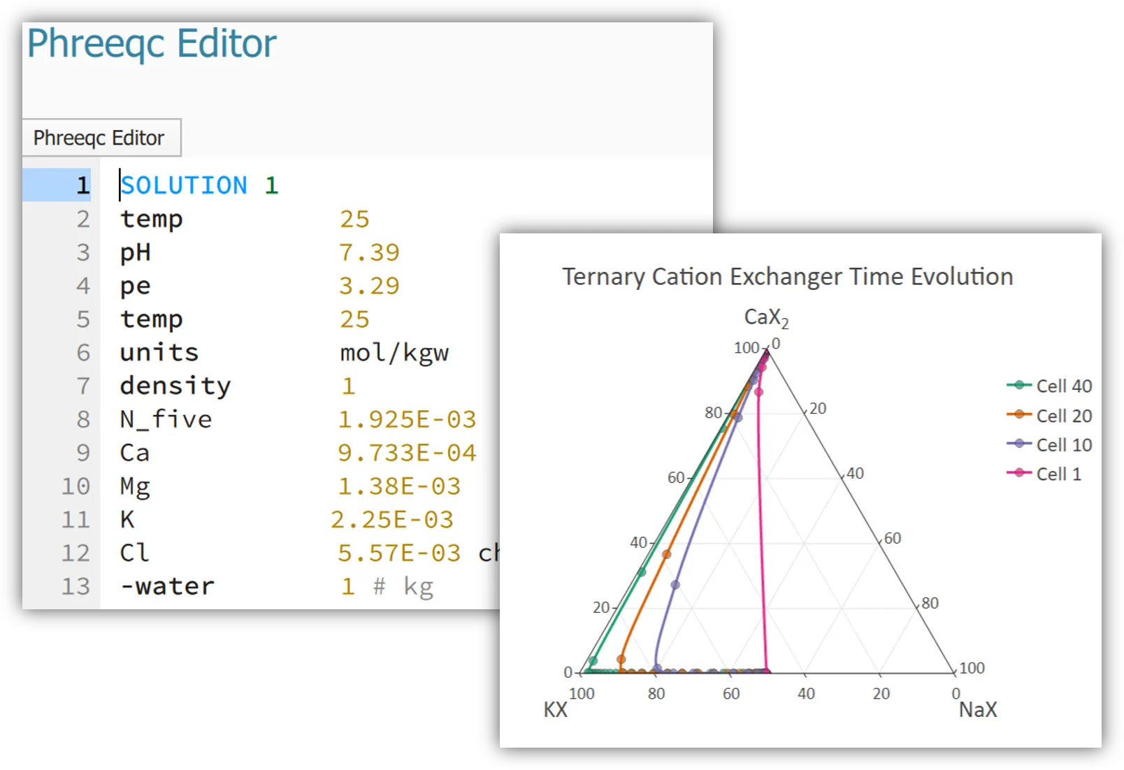
- Phreeqc Lab. Edit PHREEQC inputs with keyword autocomplete, manage thermodynamic databases and selected output definitions in one place.
- Parameterized inputs. Replace any value in an input with a parameter or a mathematical expression, then run the model for every combination you need.
- Phreeqc Study. Every run keeps its output files and selected output tables, ready to filter, tabulate and plot without copying data around.
- Your existing models. Import existing .pqi inputs and databases as they are, or drop a PHREEQC input on the window: it opens as a new project with its selected output already in a lab. GibbsStudio uses the original PHREEQC engine and saves the original output.
Pr · Pro
Predominance
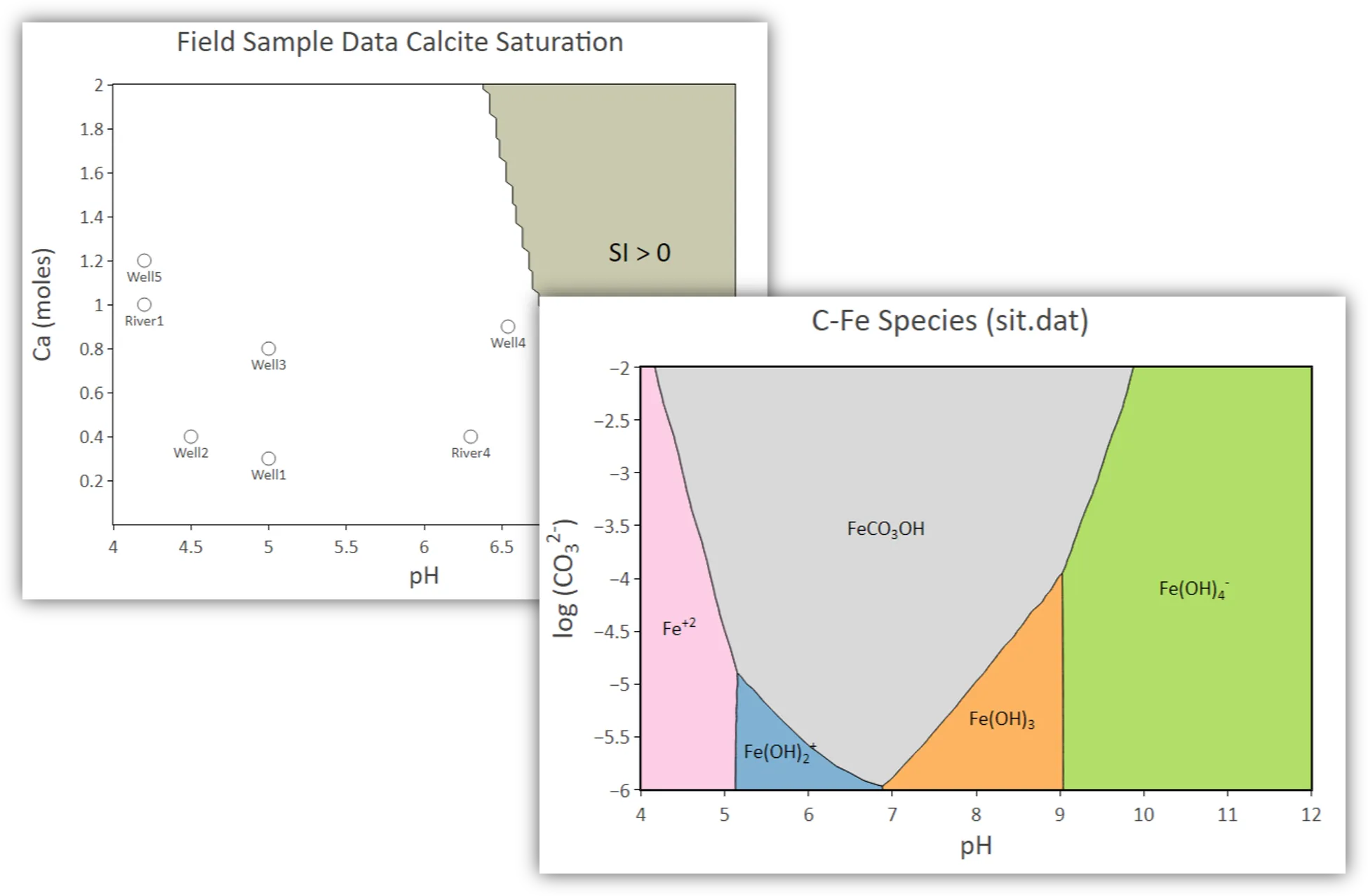
Compute predominance boundaries directly from PHREEQC and draw them as Pourbaix and stability diagrams.
- Track boundaries, not the whole field. A predominance study follows the lines where one expression gives way to another instead of evaluating everything either side of them, so a sharp diagram costs a fraction of the simulations a lattice of the same sharpness would need.
- Any two axes. Classically pe against pH — an Eh–pH or Pourbaix diagram — but the axes can be anything the model depends on: temperature, a total concentration, a partial pressure.
- Second and third rank. Each expression is reported at a level: predominant, sub-predominant, sub-sub-predominant. A species that never dominates anywhere can still be the interesting one.
- Masks, labels and your samples. Constraint areas restrict the diagram to where it means something — the water stability limits are the usual case — labels name the fields, and scatter traces put your field samples on top.
St · Pro
Statistics
Quantify how uncertain inputs propagate through your PHREEQC model, and reduce complex datasets to what matters.
- Monte Carlo study. Run PHREEQC thousands of times with inputs drawn from statistical distributions, and see the spread of every result.
- Random or Latin hypercube. Random sampling draws each simulation independently; Latin hypercube cuts each distribution into equally probable strata and draws once in each, which covers the input space with far fewer runs.
- A run you can repeat. Every study carries a seed, and the same seed draws the same samples — so a figure in a paper can be reproduced. Set it to 0 for a new draw each run. Each distribution has its own stream.
- The distributions you need. Normal, lognormal, log10-normal, truncated normal, uniform, log-uniform and triangular, one per parameter.
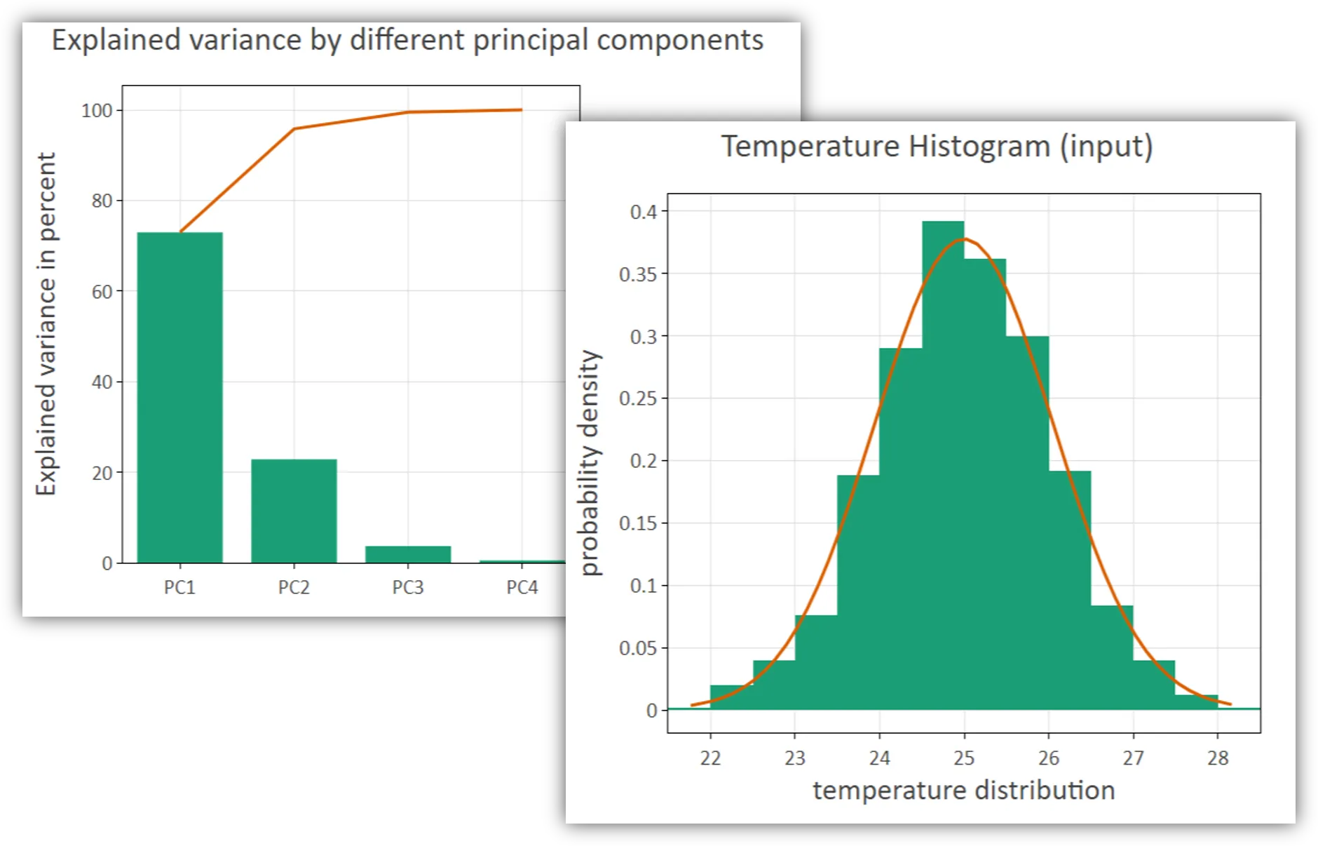
- Univariate statistics. Compute descriptive statistics and histograms for any variable in your samples or model output.
- Principal component analysis. Understand and reduce the complexity of large hydrochemical datasets with PCA.
Op · Pro
Optimization
Calibrate PHREEQC models against measurements with a least-squares solver, instead of adjusting parameters by hand.
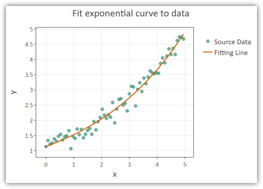
- Fitting study. Minimize a function or fit PHREEQC parameters to measured data with Ceres Solver and its trust-region methods, Levenberg–Marquardt or dogleg.
- Any parameter, any target. Fit rate constants, sorption parameters or exchange capacities against any column of your measured data, scalar or vector.
- Control over the search. Bounds keep the fit physically sensible, a parameter can be held fixed or searched on a log scale, and residuals of different reliability can be weighted by their standard deviation.
- The fit is a value. The study keeps the target run at the best parameters found, and each fitted value can be used in an expression downstream rather than copied by hand.
Db · Pro
Database
The database decides the answer as much as the input does. Look inside one, and put several side by side over the system you actually care about.
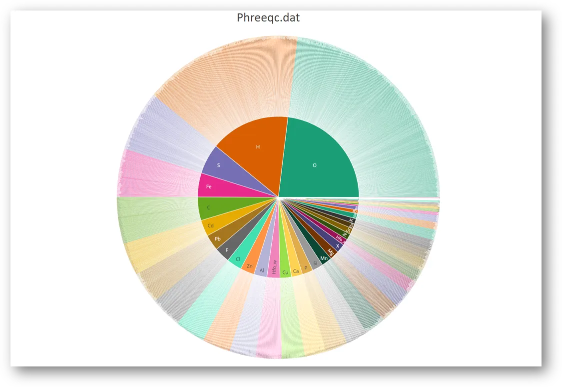
- Hierarchical views. Sunburst, treemap and icicle plots of the elements, valence states, species and phases in a PHREEQC database — how to answer "does this database have what I need?" without reading a 5 MB text file.
- Compare over a system you name. Give the comparison several databases and the elements involved — Ca, C, Fe(3) — and it reports what each database has and lacks for that system, and the species and phases per element and valence state.
- Where the numbers disagree. Where the same reaction is written alike in two databases, the comparison shows how far apart their log K values are, and plots log K against temperature. The size of the disagreement, before you meet it as a discrepancy between two projects.
- Databases travel with the project. A database is stored inside the project, not referenced from disk, so a project you send someone carries the thermodynamics it was run against.
Bring your existing PHREEQC models
Inputs and databases import as they are. PHREEQC is bundled, so you can start in minutes.